The St. Petersburg Paradox: Expected Value vs. Survival in the Real World
In 1738, Swiss mathematician Daniel Bernoulli presented a deceptively simple coin-toss puzzle to the Imperial Academy of Sciences in Saint Petersburg.
The game works as follows:
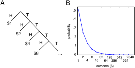
- A fair coin is tossed until the first “Heads” appears.
- If Heads appears on toss 1, you win $2.
- If Heads appears on toss 2, you win $4.
- If Heads appears on toss 3, you win $8.
- In general, if the first Heads appears on toss k, the payoff is 2^k.
Classical probability theory dictates that the fair price to enter any wager is its Expected Value E[X]. Calculating the mathematical expectation of Bernoulli’s game yields a startling result:
The theoretical expected payoff is infinite.
According to standard classical economics, a rational participant should be willing to wager their entire net worth—millions or billions of dollars—just to play this game once. Yet, in experimental trials, almost no sane human is willing to pay more than $20 to $25 to enter.
This fundamental contradiction is the St. Petersburg Paradox. It exposes the catastrophic failure of raw expected value E[X] when applied to real-world risk management, capital allocation, and derivatives trading.
The Probability Trap: The Anatomy of Infinite Expectation
Why does the game promise infinite riches on paper while delivering mediocre results in practice?
The secret lies in the distribution of outcomes:
- Toss 1 (50% probability): You win $2.
- Toss 2 (25% probability): You win $4.
- Toss 3 (12.5% probability): You win $8.
- Toss 4 (6.25% probability): You win $16.
Notice that 87.5% of the time, the game ends in 3 tosses or fewer, paying out $8 or less. Over 99% of all trials terminate before toss 7, paying out $64 or less.
The entire “infinite” expected value is driven by astronomical payouts occurring with near-zero probabilities (e.g., winning $1,073,741,824 on toss 30 with a 1-in-a-billion chance). Standard expected value calculations implicitly assume you can play an infinite ensemble of games simultaneously—the exact fallacy explored in non-ergodic systems.
Bernoulli’s Resolution: Expected Utility & Logarithmic Wealth
Daniel Bernoulli solved the paradox by separating monetary value from utility (subjective satisfaction or survival value). He argued that an additional dollar means far more to someone with an empty wallet than to someone who already possesses a fortune.
Bernoulli proposed that utility scales logarithmically with total wealth ($W$):
$$U(W) = \ln(W)$$
When you evaluate the St. Petersburg game using expected utility rather than nominal dollars, the infinite sum collapses into a modest, finite number. An individual with $1,000 in baseline wealth evaluating the game via logarithmic utility calculates an equilibrium entry price of roughly $10 to $11—aligning theory with human behavior.
This logarithmic utility function laid the mathematical foundation for modern portfolio optimization and John Kelly’s derivation of the Kelly Criterion.
The Finite Bankroll Problem: Absorbing Boundaries in Real Markets
The assumption of infinite expected value relies on a silent, impossible condition: the casino must possess infinite wealth.
In the real world, every casino, market maker, and clearinghouse operates with finite capital (C). If the house runs out of money at C = 2^M, the payoff caps out:
Consider a casino with a staggering bankroll of $1,000,000,000 (~2^{30}):
- $M = 30$
- The true mathematical expected value drops from \infty to just $31.00.
If the casino only has 1,048,576 (2^{20}), the expected value is merely $21.00.
The moment you introduce finite counterparty limits and absorbing barriers, the illusion of infinite wealth vanishes.
Trading Application: Deep OTM Options as St. Petersburg Lotteries
In financial markets, retail options buyers routinely step directly into the St. Petersburg trap.
Consider deep Out-of-the-Money (OTM) call options on volatile indices or meme stocks:
- The Pitch: “Pay ₹5. If the index moves 10%, this contract goes to ₹500 (100x payoff)!”
- The Reality: The retail trader looks at the massive tail payoff and rationalizes a positive expected value, ignoring the reality of fat-tailed distributions in Extremistan.
Because implied volatility skew inflates the cost of out-of-the-money strikes, retail participants repeatedly pay ₹5 for lotteries whose true finite expected value is less than ₹1.50 after factoring in theta decay, counterparty spread extraction, and the market for lemons adverse selection drag.
The buyer’s capital decays along a single path to zero long before the 1-in-a-million payoff arrives.
Expected Value vs. Real-World Decision Making
| Dimension | Classical Expected Value (E[X]) | St. Petersburg Reality (Real Markets) |
| Expected Payoff | Mathematically infinite (\infty) | Strictly finite ($15–$35 under real capital caps) |
| Probability Mechanics | Assumes ensemble averaging across parallel universes | Governed by single-path time averages (Non-Ergodic) |
| Counterparty Solvency | Assumes dealer has infinite liquidity | Bounded by broker/exchange capital limits |
| Value Function | Linear ($1 is always worth $1) | Concave / Logarithmic (Diminishing marginal utility) |
| Retail Vulnerability | Overpaying for theoretical expectation | Capital bleeding into an absorbing barrier ($0 ruin) |
3 Risk Rules for Quantitative Traders
1. Never Price Trades on Raw Expected Value Alone
Expected value is an ensemble metric. If a trading strategy requires thousands of repetitions or an astronomical single payoff to generate positive expectancy, an individual trader will likely hit an absorbing barrier ($0) long before the distribution converges.
2. Cap Payoff Assumptions at Counterparty Solvency
When structuring asymmetric or tail-risk hedges, never assume infinite payoff potential. Cap your model assumptions at realistic liquidity limits: exchange circuit filters, market maker capital, or broker margin boundaries.
3. Size for Geometric Growth, Not Arithmetic Averages
Because utility scales logarithmically with capital, portfolio sizing must prioritize maximizing the long-term compounding rate (geometric growth) rather than arithmetic expected profit per trade. Using fractional Kelly sizing naturally adjusts for the concave utility curve of real wealth.
Frequently Asked Questions (FAQ)
What is the core contradiction of the St. Petersburg Paradox?
The paradox is the conflict between probability theory and practical human behavior: while mathematical expected value calculates that a rational person should pay an infinite sum to play the game, no real person will pay more than a modest amount ($20–$25) due to the negligible probability of surviving past the first few tosses.
How did Daniel Bernoulli solve the paradox?
Bernoulli solved it by introducing the concept of marginal utility. He proved that wealth provides diminishing satisfaction the more you acquire, modeling utility as a logarithmic function ($U(W) = \ln(W)$). Under logarithmic utility, the expected utility of the game becomes finite.
How does the St. Petersburg Paradox apply to algorithmic trading?
In algorithmic trading, strategies that rely on rare, massive outlier gains (like lottery-type long options or grid recovery systems) often fail because the algorithm’s capital cannot survive the long drawdowns between payouts. The theoretical infinite expectation is eliminated by real-world friction, margin calls, and finite account balances.