Fat Tails & The Ludic Fallacy: Why Financial Models Fail in Extremistan
Financial markets operate in Extremistan, where power laws and fat tails render thin-tailed Gaussian models like VaR and Sharpe ratios useless. Mistaking messy markets for predictable casino games—the Ludic Fallacy—causes ruin. To survive, traders must abandon fragile optimization, haircut position sizing, and deploy convex Barbell structures that guarantee survival through liquidity black holes.
By Suyesh Gusain (B.Sc. Physics Hons., NISM Certified Research Analyst & Equity Derivatives)
Disclaimer: This article is strictly for educational, statistical, and quantitative risk analysis. It does not constitute financial, investment, or trading advice.
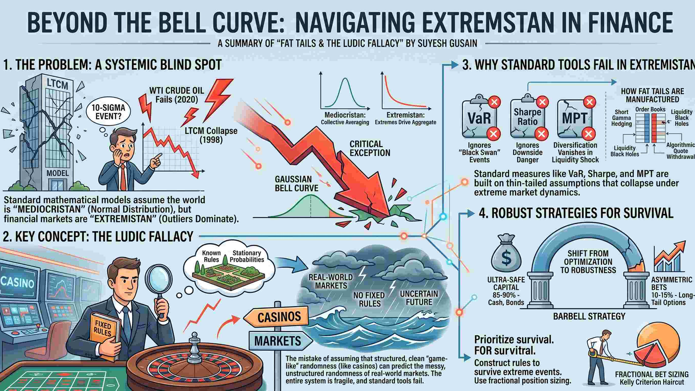
In 1998, Long-Term Capital Management (LTCM)—a fund led by Wall Street titans alongside Nobel Memorial Prize-winning economists Robert Merton and Myron Scholes—lost $4.6 billion in under four months.
Their mathematical risk models calculated that the sequence of events triggering their collapse was a “10-sigma event”—something statistically projected to happen roughly once every few million years. The fund collapsed in less than five.
Twelve years later, on April 20, 2020, West Texas Intermediate (WTI) crude oil futures plummeted below zero to settle at -$37.63 per barrel. Conventional Gaussian option pricing algorithms on major commodity exchanges broke instantly because they assumed energy asset prices followed log-normal distributions where absolute prices cannot fall below zero.
The systemic blind spot that broke LTCM, shattered energy models in 2020, and repeatedly liquidates derivative portfolios stems from a single error: treating financial markets as if they belong to Mediocristan (the domain of the Gaussian Bell Curve) when they strictly operate in Extremistan (the domain of Power Laws and Fat Tails).
What is Extremistan?
Extremistan is a statistical environment governed by power laws and fat tails, where a single extreme outlier can disproportionately alter aggregate outcomes. Coined by Nassim Nicholas Taleb, it contrasts with Mediocristan (Gaussian distributions), describing complex, non-linear domains like financial markets, venture capital, and catastrophic risk.
In Extremistan, the concept of a “typical” event is an illusion. The aggregate is not driven by the collective average, but by the extreme outlier.
Two Statistical Worlds: Mediocristan vs. Extremistan
To understand why standard risk formulas break down, we must distinguish between two incompatible probability regimes.
1. Mediocristan (The Gaussian Domain)
In Mediocristan, randomness is dominated by the collective. Individual events lack the scale to alter the aggregate total.
- Everyday Examples: Human height, body weight, calorie consumption, or 10,000 flips of a fair coin.
- The Mathematics: If you gather 1,000 people in a room and add the heaviest individual on Earth, total sample weight shifts by a fraction of a percent. The distribution is bounded, governed by the Central Limit Theorem, and follows a thin-tailed Gaussian (normal) curve.
- The Core Metric: The sample mean (μ) and standard deviation (σ) provide meaningful, predictive measurements of probability.
2. Extremistan (The Power-Law Domain)
In Extremistan, randomness is dominated by extreme outliers. A single observation dictates the aggregate outcome.
- Everyday Examples: Wealth distribution, book sales, war casualties, and equity price movements.
- The Mathematics: If you gather 1,000 people in a room and add Elon Musk, his net worth will account for more than 99.9% of the room’s total wealth.
- The Core Metric: Standard deviation (σ) ceases to be predictive. The tail follows a Power Law (Pareto-Lévy-Mandelbrot distributions), where rare, catastrophic events dominate cumulative variance:
P(X>x)∼x−α
When the tail exponent α is low, higher statistical moments (such as variance and kurtosis) become unstable or mathematically undefined.
Mediocristan vs. Extremistan Comparison
| Dimension | Mediocristan (Standard Finance) | Extremistan (Real-World Markets) |
|---|---|---|
| Underlying Distribution | Gaussian (Normal / Bell Curve) | Power Laws, Pareto-Lévy distributions |
| Impact of a Single Event | Negligible; absorbed by sample mean | Catastrophic; can dictate total returns |
| Probability of a 5-Sigma Event | Roughly 1 in 3.5 million days (~13,000 years) | Observed every 3–5 years across asset classes |
| Reliability of Standard Deviation (σ) | High; accurately bounds variance | Unreliable; variance is driven by rare outliers |
| Tail Risk Behavior | Exponential decay (Thin tails) | Polynomial decay (Fat tails) |
| Ultimate Risk | Underestimating volatility drag | Complete liquidation / Absorbing barrier |
Python Verification: Proving Fat Tails in Market Data
In a theoretical Gaussian distribution, excess kurtosis is exactly 0 (normal kurtosis = 3). Any distribution with kurtosis significantly greater than 3 is classified as leptokurtic—confirming fat tails and high peak density.
You can verify this directly using Python and historical index data:
Python
import yfinance as yf
import scipy.stats as stats

# Fetch 15+ years of index data (e.g., S&P 500 or Nifty 50)
data = yf.download('^GSPC', start='2005-01-01')['Close']
log_returns = (data / data.shift(1)).dropna()

# Compute Kurtosis (Gaussian = 3.0)
kurt_value = stats.kurtosis(log_returns, fisher=False)
print(f"Empirical Kurtosis: {kurt_value:.2f}")
# Output typically exceeds 10.0 to 25.0+ depending on the lookback window,
# mathematically refuting the Gaussian distribution assumption.
When empirical kurtosis exceeds 10, relying on normal distribution standard deviation is not just suboptimal—it is mathematically invalid.
The Ludic Fallacy: Why Casinos Are Not Markets
The Latin word for game is ludus. Nassim Nicholas Taleb defines the Ludic Fallacy as the mistaken belief that the clean, well-defined randomness of games and casinos can map onto the unstructured, messy randomness of real life.
In a casino:
- The rules are fixed and immutable.
- The sample space of outcomes is completely known (e.g., exactly 37 or 38 pockets on a roulette wheel).
- Probabilities are stationary and ergodic.
Financial markets, however, are open, reflexive, and non-stationary. When risk models treat markets like casinos, they assume the worst possible loss is bounded by the parameters of the game. In reality, market rules change dynamically, liquidity vanishes, and counterparties default.
The Fatal Flaws of Standard Finance: VaR, Sharpe Ratio, and MPT
Mainstream financial engineering relies on three primary tools built on thin-tailed assumptions. In Extremistan, each tool fails systematically:
- Value at Risk (VaR): VaR measures potential losses up to a threshold (e.g., “We are 99% confident we will not lose more than $2M today”). The fatal flaw: VaR ignores the remaining 1%. In Extremistan, that 1% contains black swans that can wipe out decades of capital in a single morning.
- The Sharpe Ratio: By dividing excess returns by standard deviation (σ), the Sharpe ratio treats upside volatility and downside volatility as equally harmful. More dangerously, strategies that sell deep out-of-the-money options show near-flawless historical Sharpe ratios—right up until a gap move causes an irreversible blowout.
- Modern Portfolio Theory (MPT): Markowitz’s mean-variance optimization assumes stable cross-asset covariance matrices. In a liquidity shock, asset correlations snap toward 1.0. Diversification disappears precisely when the portfolio needs it most.
How Liquidity Black Holes Create Fat Tails
Fat tails are not just abstract statistical formulas—they are manufactured by the mechanics of the order book:
- Short Gamma Hedging: Options market makers who are short volatility must dynamically sell as prices plummet to maintain delta-neutral books, compounding downward momentum.
- VPIN Toxicity Spikes: When toxicity metrics like VPIN surge, algorithmic market makers withdraw quotes to avoid the market for lemons trap.
- Air Pockets: With passive limit orders cancelled, incoming market sell orders drop through empty order books, creating instantaneous multi-percent gaps that standard Gaussian models classify as “statistically impossible.”
Quantitative Risk Management: How to Trade Fat-Tailed Markets
1. Shift from Optimization to Robustness
Stop tweaking indicators to maximize backtested Sharpe ratios. An over-optimized system is fragile in Extremistan. Prioritize survival: construct rules so that no gap opening, black swan, or broker failure can push your equity into an absorbing barrier ($0 capital).
2. Implement the Barbell Strategy
The Barbell Strategy replaces the fragile “moderate-risk” middle ground with two distinct poles:
- 85% to 90% in Ultra-Safe Capital: Cash equivalents, short-term sovereign paper, or risk-free liquid reserves completely shielded from market crashes.
- 10% to 15% in Asymmetric Convex Bets: High-upside instruments with strictly defined maximum downside (e.g., long tail-risk options, convex trend following, early-stage venture setups).
This structure caps your maximum drawdown while leaving your portfolio exposed to positive outliers.
3. Haircut Your Position Sizing
Mathematical bet sizing formulas like the Kelly Criterion assume known, stationary probabilities. Because real-world drawdown distributions are governed by power laws, using full-Kelly sizing guarantees liquidation over a long enough time horizon. Using fractional sizing (such as quarter-Kelly or eighth-Kelly) provides the essential buffer required to survive Extremistan.
Frequently Asked Questions (FAQ)
What makes a distribution “fat-tailed”?
A distribution is fat-tailed (or heavy-tailed) when extreme outcomes have a significantly higher probability of occurring than predicted by a normal (Gaussian) distribution. Tail probabilities decay polynomially (x−α) rather than exponentially (e−x2), meaning outliers continue to drive aggregate variance.
How does the Ludic Fallacy harm options traders?
Traders commit the Ludic Fallacy when they assume options pricing frameworks (like Black-Scholes) describe reality rather than an idealized model. Because Black-Scholes assumes continuous price paths and Gaussian log-returns, it systematically underprices deep out-of-the-money tail risk, encouraging option sellers to pick up nickels in front of steamrollers.
Why do “10-sigma events” occur so often in financial markets?
Under a Gaussian bell curve, a 10-sigma event is statistically impossible over the age of the universe. When financial crashes (such as 1987, 1998, 2008, or 2020) are labeled “10-sigma events,” the market didn’t break mathematics—the analyst used the wrong model. In an Extremistan power-law distribution, events of that scale occur regularly.